Capon Heatmap Processor

Introduction

The Capon heatmap processor — also known as the Minimum Variance Distortionless Response (MVDR) beamformer — replaces the Bartlett quadratic form with the reciprocal of \(\mathbf{a}^H R^{-1} \mathbf{a}\). The result is a much narrower main lobe than the conventional beamformer for the same array aperture, at the cost of inverting the channel covariance matrix at every range bin and being sensitive to mismatch between the assumed steering vector and the true channel response. This mismatch is small enough, in practice, for Capon to perform reliably as a DOA estimator. The small residual mainly affects amplitude estimates; see Robust Capon.

Typical use case

• High-resolution direction-of-arrival applications where two or more closely spaced targets must be resolved.

• Applications with many targets whose side lobes could mask each other when using conventional beamforming.

• When the application only demands DOA estimates (no power estimate) and SNR is good. Because A212 uses offline steering-vector calibration, the accuracy is not high enough to use Capon as an amplitude estimator. The accuracy of the calibration is, however, high enough to use it as a high-performance DOA estimator. (See robust Capon.)

• As the input to a CFAR detector — Capon’s narrow main lobes and low side lobes give clean peaks for adaptive thresholding.

Pros and cons

Pros

• Markedly higher angular resolution than conventional beamforming.

• Lower side lobes and noise level; better at finding and separating targets.

• Lower spectrum variance.

• Adaptive: nulls on strong interference.

Cons

• Requires inverting \(R\) at every range bin every frame — more expensive than conventional.

• Sensitive to steering-vector mismatch: not suited for amplitude estimation. (See Robust Capon for amplitude workaround.)

• The number of samples used for one heatmap needs to exceed the number of channels used. This is needed to ensure that the covariance matrix is invertible.

• Sensitive to low SNR.

Math and theory

Let \(R \in \mathbb{C}^{N_{ch} \times N_{ch}}\) be the smoothed estimate of the channel covariance matrix at a given range bin and \(\mathbf{a}(\theta, \phi) \in \mathbb{C}^{N_{ch}}\) the steering vector for direction \((\theta, \phi)\). The Capon (MVDR) output is

\[P_{\text{capon}}(\theta, \phi) = \frac{1}{\mathbf{a}(\theta, \phi)^H R^{-1} \mathbf{a}(\theta, \phi)}.\]

This corresponds to the optimization problem of minimizing the output power subject to a unit-gain constraint in the steering direction, which both sharpens peaks on real targets and suppresses energy arriving from other directions (interference). See P. Stoica and R. Moses, Spectral Analysis of Signals (Prentice Hall, 2005) for the full derivation.

Example spectrum plots

Compared to Conventional, Capon gives well-separated peaks for the three targets. The amplitude of the peaks does, however, correlate poorly with the actual amplitude of the signals.

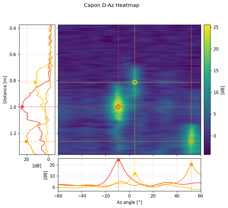
Figure 52 Capon D–Az heatmap on a recording of three corner reflectors. The three colored markers and dashed lines mark the true reflector locations. The 1D plots show the distance and azimuth spectra cut at each of the three true peak locations. Recorded using Profile 3.

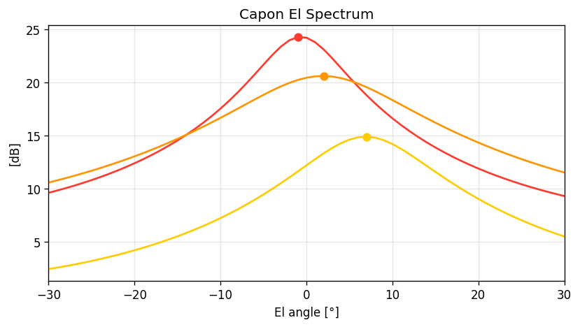
Figure 53 Elevation spectrum of the Capon heatmap at each of the three true peak locations. Recorded using Profile 3.

Configuration

Shared parameters are documented in Shared Heatmap Configuration. Processor-specific fields:

covariance_matrix_time_constant_s

Time constant of the exponential smoothing applied to the per-range covariance matrices across frames. Capon is more sensitive to a noisy \(R\) than the conventional processor, so this parameter typically deserves more care. See the shared notes for more tuning guidance.

high_pass_filter_time_constant_s

Time constant of the per-channel high-pass filter that runs on the IQ data to suppress static signals before the covariance is built. The Capon processor always runs this filter since it cannot handle perfectly correlated signals (static signals will always be perfectly correlated). See the shared notes for more tuning guidance.

Typical processing cost

Per frame, the Capon processor does everything the conventional processor does, plus a per-range matrix inverse (\(\mathcal{O}(N_d \cdot N_{ch}^3)\)). Beyond that, the beamforming quadratic form is structurally the same as in conventional. On the configuration the RSS computation time test measures, 12 virtual channels and 25 azimuth angles, this corresponds to ~1.5 × the per-frame cost of Conventional.

API reference

class acconeer.exptool.a2.algo.heatmap.capon.HeatmapProcessor(subsweep_config: SubsweepConfig, heatmap_config: HeatmapConfig, update_rate: float)

process(result: Result) → ProcessorResultCommon

Process a SparseIQ Result

Initializes internal state the first num_channels frames.

class acconeer.exptool.a2.algo.heatmap.capon.HeatmapConfig(antenna_array, az_angle_range: t.Any, el_angle_range: t.Any, num_az_angles: int, num_el_angles: int, covariance_matrix_time_constant_s: float, high_pass_filter_time_constant_s: float)

covariance_matrix_time_constant_s: float

Time constant for exponential smoothing of the covariance matrices

high_pass_filter_time_constant_s: float

Time constant for the high-pass filter.

classmethod default() → Self