Heatmap

A heatmap is a 3-D power map indexed by (distance, azimuth, elevation) produced by beamforming the multi-channel sweep across a configured angular grid. The A212 stack provides four heatmap processors that differ only in the beamforming step they use to map the channel data (or its covariance) into that grid.

The processors provide baseline beamforming examples. Typical usage often needs to adapt the methods to the use case with varying pre- and post-processing.

This section documents each processor and the shared configuration base.

Picking a processor

Processor	Input to beamformer	Resolution	Robustness to steering-vector mismatch	Relative numerical cost
Coherent	Channel data (complex)	Lowest	n/a (no statistics)	~0.3 × (estimate)
Conventional	Channel covariance	Baseline	High (wide main-lobe)	1 × (baseline)
Capon	Channel covariance	High	Low (sensitive to mismatch)	~1.2 ×
Robust Capon	Channel covariance	High (slightly broader than Capon)	High (configurable via steering_vector_epsilon)	~3.5 ×

The ratios are stable across configurations because the beamforming step dominates the covariance update by roughly an order of magnitude.

Capon’s Low rating reflects the algorithmic sensitivity to mismatch. The residual mismatch is small in practice, so Capon is a reliable DOA estimator. The small residual mainly affects amplitude estimates — when those matter, see Robust Capon.

Shared processing pipeline

All four processors apply the same preparation steps before their distinguishing beamformer runs:

1. Mean across sweeps in the frame, leaving one complex value per (distance, channel).

2. Optional per-channel high-pass filter (MovementNode). Always on for Capon and Robust Capon; toggleable via heatmap_mode for Coherent and Conventional.

3. Reshape to (num_points, num_channels).

4. Channel covariance along the channel axis, shape (num_points, num_channels, num_channels) — skipped by Coherent.

5. Exponential smoothing of the covariance matrices across frames — skipped by Coherent.

6. Beamforming on the angular grid — the main difference between the four processors. See each processor page for more details.

The output is always a heatmap array of shape (num_points, num_az_angles, num_el_angles).

Beamformer comparison

Figure 45 and Figure 46 overlay the four beamformers on the same recording of a corner reflector. Both 1D cut figures are taken at the known true corner reflector location. The output of the Coherent heatmap is an amplitude, \(|y|\), while the others are powers, \(|y|^2\); the coherent line is therefore squared before the overlay, so all four are on the same power scale.

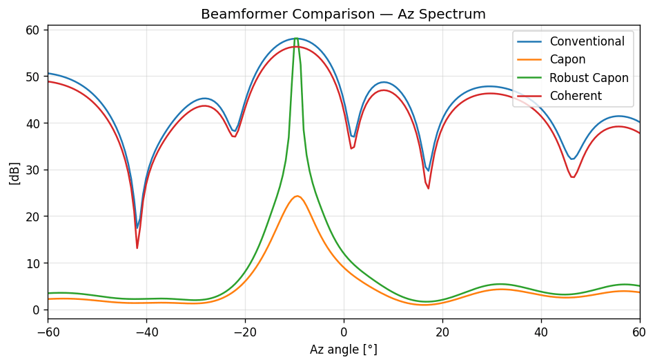
Figure 45 Azimuth cut through the strongest reflector for all four beamformers. Capon and robust Capon show the narrowest main lobes; conventional and coherent have the widest. Recorded using Profile 3; robust Capon with \(\varepsilon = 0.02\).

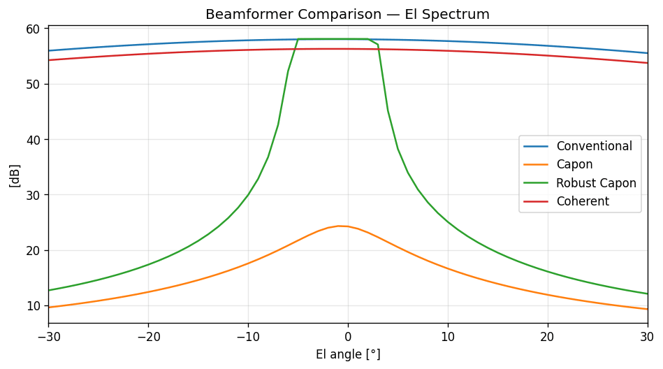
Figure 46 Elevation cut through the strongest reflector for all four beamformers. Recorded using Profile 3; robust Capon with \(\varepsilon = 0.02\). Since the A212 has an array width of only two channels in elevation, the elevation spectrum cannot separate multiple targets — it can only localize a single one.

Configuration

The base class HeatmapConfigCommon covers the fields used by every processor and is documented separately in Shared Heatmap Configuration. Two more parameters are worth mentioning since they appear in all processors except the coherent one:

Covariance smoothing low-pass filter. The covariance-based processors (Conventional, Capon, Robust Capon) maintain an exponentially smoothed estimate of the channel covariance matrix \(R\) across frames. The time constant is set by covariance_matrix_time_constant_s. Longer time constant gives a less noisy \(R\) but lag moving targets; shorter values follow motion more quickly at the cost of more frame-to-frame variation in the heatmap. Capon and Robust Capon are more sensitive to a noisy \(R\) than the conventional processor and typically benefit from a slightly longer time constant. The apparent number of samples in the estimate is determined both by covariance_matrix_time_constant_s and the update_rate. Increasing update_rate can give higher smoothing without increasing the filter lag at the cost of higher power consumption.

Per-channel IQ high-pass filter. Before the covariance is built, an exponential high-pass filter can be applied to each channel’s IQ data to suppress the static scene. The time constant is set by high_pass_filter_time_constant_s. A longer time constant will suppress slow moving objects less at the cost of slower adaption to static objects that change position. Setting the value to 0 will give a two-pulse canceller filter, i.e., the previous frame is subtracted from the current one.

Exploration Tool

The four heatmap processors are exposed in Exploration Tool with three plot tabs that share the same underlying heatmap data:

• Cartesian — 2-D distance–azimuth heatmap on Cartesian axes.

• Polar — the same 2-D distance–azimuth heatmap in polar coordinates.

• 3D view — 3-D scatter of the thresholded heatmap in \((d, \text{az}, \text{el})\). The threshold is set by normalized_heat_cutoff.

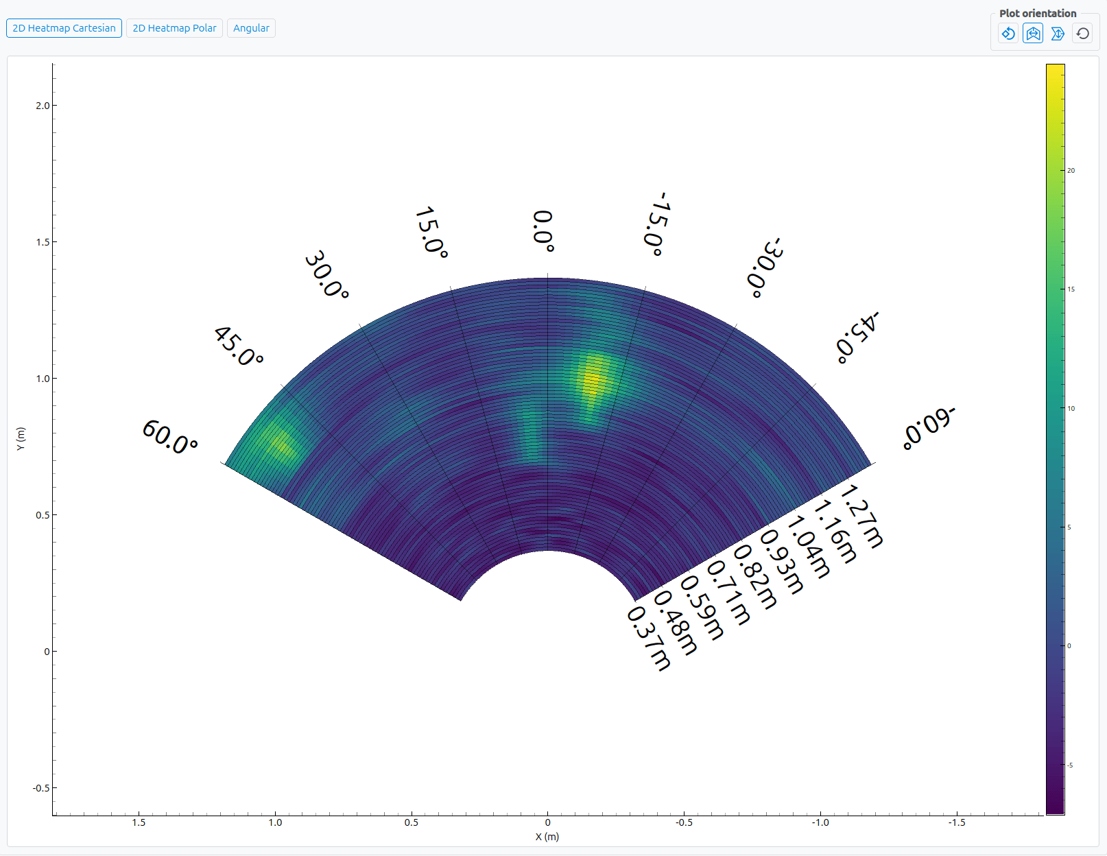
Figure 47 The Cartesian heatmap tab in Exploration Tool. The three tab buttons at the top — 2D Heatmap, 2D Heatmap Polar, 3D view — switch between the views; the Plot orientation controls on the right rotate the sensor frame.

• Shared configuration
• Coherent
• Conventional
• Capon
• Robust Capon
• Channel corrections