Coherent Heatmap Processor

Introduction

The coherent heatmap processor implements the classic delay-and-sum beamformer directly on the per-channel data. For each point on the (distance, azimuth, elevation) grid it computes a single complex value — the sum of the channel signals phase-aligned to that direction. The magnitude or phase of that complex value forms the heatmap that is displayed in ET; the underlying complex array is also exposed in ProcessorResult.

Unlike the three covariance-based processors — Conventional, Capon, and Robust Capon — the coherent processor does not estimate a channel covariance matrix and does not invert one. This makes it the cheapest option and the only one that preserves the phase information. Conventional beamforming is equivalent to the coherent beamforming with averaging of heatmaps over time. The difference is that conventional beamforming achieves higher numerical efficiency by averaging at the covariance level when done over many snapshots.

Typical use case

• Pipelines downstream of the heatmap that need the complex output — for example, micro-Doppler or phase-tracking applications, such as vital sign applications.

Pros and cons

Pros

• Cheapest of the four processors; no covariance, no matrix inverse. But it is often used in phase-tracking applications where a higher heatmap update rate is desirable.

• Can image static scenes — unlike Capon it handles correlated sources.

• Provides complex output, which retains phase information.

• No covariance smoothing — responsive to fast scene changes.

Cons

• Angular resolution is limited by the array aperture. FWHM \(\approx 10.2 ^\circ\) at boresight; broadens off-boresight as the effective aperture scales with \(\cos\theta\).

• High side lobe levels; side lobes leak energy from strong reflectors into other directions.

• No averaging over time — higher spectrum variance.

Math and theory

Let \(\mathbf{x} \in \mathbb{C}^{N_{ch}}\) be the channel data at a given range bin (after the optional high-pass filter, taken from the time-averaged sweep) and \(\mathbf{a}(\theta, \phi) \in \mathbb{C}^{N_{ch}}\) the steering vector for direction \((\theta, \phi)\). The delay-and-sum output is

\[y(\theta, \phi) = \mathbf{a}(\theta, \phi)^H \mathbf{x}.\]

The processor produces the complex array \(y(\theta, \phi)\) for every range bin (the heatmap_coherent output) and a real heatmap selected from it by display_mode: either \(|y|\) (ABSOLUTE) or \(\arg(y)\) (ANGLE).

Example spectrum plots

As seen in Figure 48, the sidelobes of the actual targets can mask other weaker reflectors. A peak-finding algorithm would not be able to find the three positions. The beamforming method can, however, still be used for amplitude estimation and phase extraction applications.

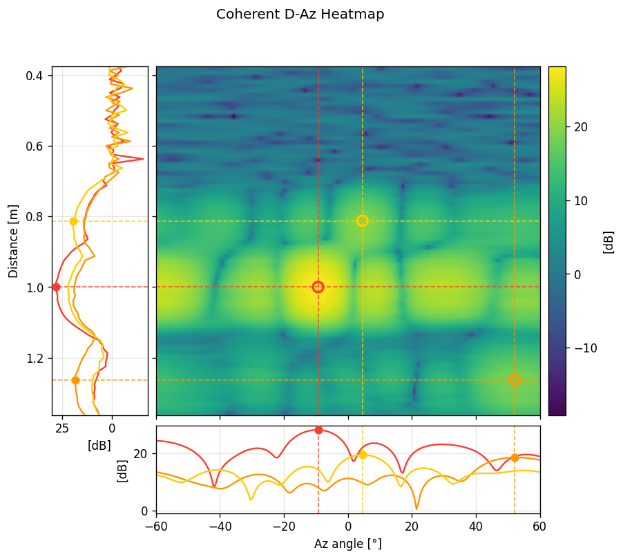
Figure 48 Coherent D–Az heatmap on a recording of three corner reflectors, plotted as \(|y|\). The three colored markers and dashed lines mark the true reflector locations. The 1D plots show the distance and azimuth spectra cut at each of the three true peak locations. Recorded using Profile 3.

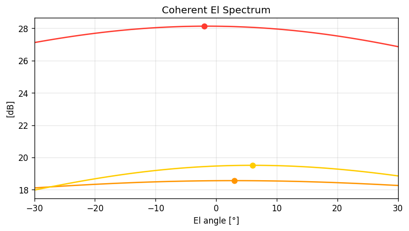
Figure 49 Elevation spectrum of the coherent heatmap at each of the three true peak locations. Recorded using Profile 3.

Configuration

Shared parameters are documented in Shared Heatmap Configuration. Processor-specific fields:

heatmap_mode

MOVEMENT enables a per-channel high-pass filter that suppresses the static scene; DISTANCE skips the filter and shows the full reflected energy.

high_pass_filter_time_constant_s

Time constant of the high-pass filter when heatmap_mode is MOVEMENT. Ignored otherwise.

display_mode

Lives on CoherentHeatmapPlotConfig (see also the shared Shared Heatmap Configuration page). Selects what the real heatmap output contains: ABSOLUTE for the magnitude of the complex beamformer output, ANGLE for its phase. The full complex array is always exposed separately as heatmap_coherent.

Typical processing cost

Per frame the processing is dominated by the beamforming step itself, \(\mathcal{O}(N_d \cdot N_{ch} \cdot N_{az} \cdot N_{el})\) complex multiplications and additions. No covariance matrix is calculated or inverted. This is the cheapest of the four processors. On the configuration the RSS computation time test measures, 12 virtual channels and 25 azimuth angles, it is 0.16 × the per-frame cost of Conventional.

On the other hand, using the coherent beamformer often implies a higher sweeps_per_frame or update_rate in order to observe phase changes over time, which adds to the total processing cost per second.

API reference

class acconeer.exptool.a2.algo.heatmap.coherent.HeatmapProcessor(subsweep_config: SubsweepConfig, heatmap_config: HeatmapConfig, update_rate: float, display_mode: DisplayMode = DisplayMode.ANGLE)

process(result: Result) → ProcessorResult

Process a SparseIQ Result

Initializes internal state the first num_channels frames, then returns a heatmap every update_count frames.

class acconeer.exptool.a2.algo.heatmap.coherent.HeatmapConfig(antenna_array, az_angle_range: t.Any, el_angle_range: t.Any, num_az_angles: int, num_el_angles: int, heatmap_mode, high_pass_filter_time_constant_s: float)

class HeatmapMode(*values)

Heatmap mode. MOVEMENT high-pass filters data. DISTANCE does no filtering

DISTANCE = 1

MOVEMENT = 2

heatmap_mode: HeatmapMode

Heatmap mode to use

high_pass_filter_time_constant_s: float

Time constant for the high-pass filter.

classmethod default() → Self

class acconeer.exptool.a2.algo.heatmap.coherent.plot_config.CoherentHeatmapPlotConfig(normalized_heat_cutoff: float = 0.75, max_2d_heat: int | None = None, log_scale_output: bool = False, display_mode=DisplayMode.ANGLE)

class DisplayMode(*values)

Display mode. ABSOLUTE returns absolute of complex value. ANGLE returns complex argument.

ABSOLUTE = 1

ANGLE = 2

display_mode: DisplayMode

classmethod default() → Self

class acconeer.exptool.a2.algo.heatmap.coherent.ProcessorResult(*, heatmap: npt.NDArray[np.float64] | None, heatmap_config: HeatmapConfigCommon, heatmap_coherent: npt.NDArray[np.complex128] | None)

heatmap_coherent: NDArray[complex128] | None

Complex heatmap data.