A212 Integration

A212 Integration#

A212 Electrical integration#

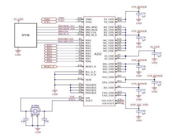
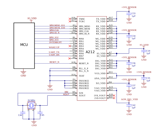
The A212 is a 60 GHz, multi-antenna radar system delivered as a one package solution with an integrated MCU, RF front-end and antennas (3TX, 4RX). To integrate it in your application, an external 26 MHz crystal, decoupling capacitors and power supply are required.

Some applications can run directly on the A212’s internal MCU, i.e. no external host is needed. For these cases an external NVM is required to boot the A212.

In production test the NVM can be flashed via the SPI (fastest), UART (slower) or the TCKC/TMSC pins (slowest).

For applications that require an external MCU host, the NVM is optional since the sensor can boot from the external MCU. See Figure A: NVM integration and Figure B: MCU integration for example integrations.

Figure A: A212 NVM integration

Figure B: A212 MCU integration

Power#

A regulator is needed to provide 1.8V and IO_VDD to the sensor. IO_VDD supports both 3.3 V and 1.8 V. The total current consumption per sensor state is specified in the table Table 1 (T_op = 25°C, nominal supplies):

Table 1 Total current consumption per sensor state#
Symbol	Parameter	Typ	Unit	Condition
I_sleep-ultra	Current consumption, SLEEP-ULTRA-DEEP state	40	µA
I_sleep-deep	Current consumption, SLEEP-DEEP state	46	µA
I_{sleep-shallow}	Current consumption, SLEEP-SHALLOW state	0.28	mA
I_idle	Current consumption, IDLE state	1.1	mA
I_processing	Current consumption, PROCESSING state	33	mA
I_measure	Current consumption, MEASURE state	174	mA	Profile 1, 2, 3, 5; PRF = 27.7 MHz
I_measure-p6	Current consumption, MEASURE state	182	mA	Profile 6; PRF = 27.7 MHz
I_full	Current consumption, FULL state	192	mA	Profile 1, 2, 3, 5; PRF = 27.7 MHz
I_full-p6	Current consumption, FULL state	200	mA	Profile 6; PRF = 27.7 MHz

Supply noise#

Noise in the power supplies may affect the performance of the A212 sensor. Table 2 provides the recommended maximum ripple levels for the DIG_VDD, RX_VDD, TX_VDD, WG_VDD, XO_VDD, VCO_VDD and ANA_VDD supplies.

Table 2 Power supply ripple specifications (T_op = 25°C)#
Frequency [kHz]	Max supply ripple [mV_pp]
50	30
100	30
200	15
300	15
500	12
750	7
1000	7
1500	5

If the voltage source violates the supply ripple specifications in Table 2, an LC filter as shown in Figure 1 can be used. This filter has a cut-off frequency of 22 kHz. You can tune the values depending on the frequency and amplitude of the ripple. Be aware of the LC filter peaking at the series resonance frequency \(f_r = \frac{1}{2\pi\sqrt{LC}}\). A small snubber resistor (250 mΩ in the example) can be inserted to lower the Q factor.

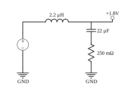
_images/A212_LC_filter.svg — Figure 1 Optional LC supply filter.#

Crystal selection#

The A212 has a built in oscillator that requires an external 26 MHz crystal. The crystal connection diagram is shown in Figure 2.

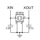
_images/A212_XTAL_connection.svg — Figure 2 Crystal (XTAL) connection diagram.#

For the oscillator to be able to drive the crystal, the following criterion must be fulfilled:

\[f_{xtal} \cdot C_L^{0.8} \cdot R_{ESR}^{0.61} < 0.7 \quad \text{(Eq. 1)}\]

where \(f_{xtal}\), \(C_L\) and \(R_{ESR}\) are defined in the crystal datasheet.

The load capacitance \(C_L\) is calculated as:

\[C_L = \frac{C'_{10} \cdot C'_{11}}{C'_{10} + C'_{11}} \quad \text{(Eq. 2)}\]

where:

\[C'_{10} = C_{10} + C_{10\text{-parasitic}} \quad \text{(Eq. 3)}\]

\[C'_{11} = C_{11} + C_{11\text{-parasitic}} \quad \text{(Eq. 4)}\]

\(C_{\text{parasitic}}\) is the PCB trace and package capacitance between the crystal pins (XIN and XOUT) and GND, expected to be between 1 pF and 2.5 pF per cm (depending on the trace width and stackup) plus package capacitance.
\(C_{10}\) and \(C_{11}\) can be calculated as:

\[C_{10} = C_{11} = 2 \cdot C_L - C_{\text{parasitic}} \quad \text{(Eq. 5)}\]

Hardware schematics design checklist#

When designing the hardware schematics for the A212 sensor, the following checklist can be used to ensure a good design:

Does the selected crystal fulfill the load conditions according to the XTAL selection?
Are all ground pins of the A212 connected on the schematic symbol?
Does the selected regulator meets the Supply noise recommendations?
Are enable and interrupt pins connected?
Have you considered how to flash the NVM/MCU during production test?

PCB guidelines#

As no RF components are required for the sensor integration, low-cost FR-4 type PCBs can generally be used. The following sections provide important information how to optimize the sensor PCB layout for good far-field directivity and side lobe level.

Component placement and routing#

The A212 sensor integrates folded dipole antennas, with the internal IC package ground plane extending beneath the entire sensor area serving as the primary ground reference. To further enhance directivity, the antenna ground plane should be extended onto the PCB by connecting all GND pads to the top copper layer. The PCB ground plane area adjacent to the sensor acts as a reflector and should therefore be a solid copper pour with minimal routing or external components, see Figure 3.

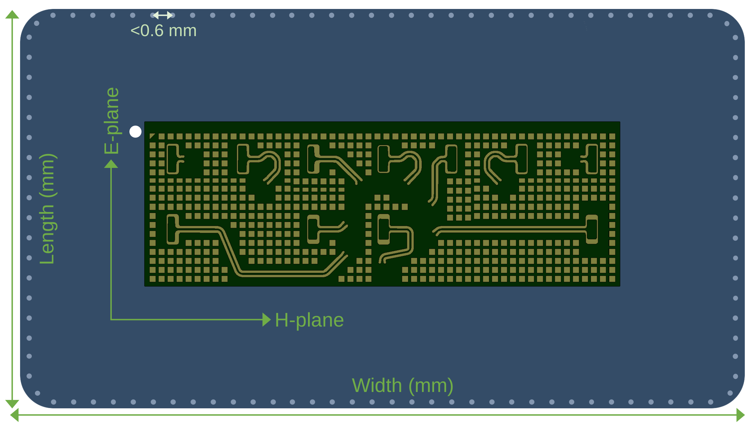
_images/A212_pcb_back_side_components_3D.svg — Figure 3 A212 on PCB with E and H-planes shown.#

External component placement#

The preferred way is to place all external components such as decoupling capacitors and crystal on the opposite side of the sensor as this typically results in the highest directivity and lowest side lobe level. In addition, to maximize the radiated performance, consider the following:

Minimize the amount of routing on the sensor layer, especially close to the sensor. This can be done by routing the signals to the sensor with vias placed as close as possible to the sensor pads, see Figure 4. The ground plane area inside the footprint has lower impact on the radiated performance and therefore some vias and short traces are preferably placed there.
Whenever the assembly process allows, remove thermal reliefs on all sensor pads.
Choose small pad size vias such as 0.4-0.45 mm or smaller.
Minimize copper clearance for traces, vias, and pads on the sensor layer to maximize the ground plane area close to the sensor.
Add stitching vias with <0.6 mm spacing at the PCB outer edge to suppress potential edge radiation.

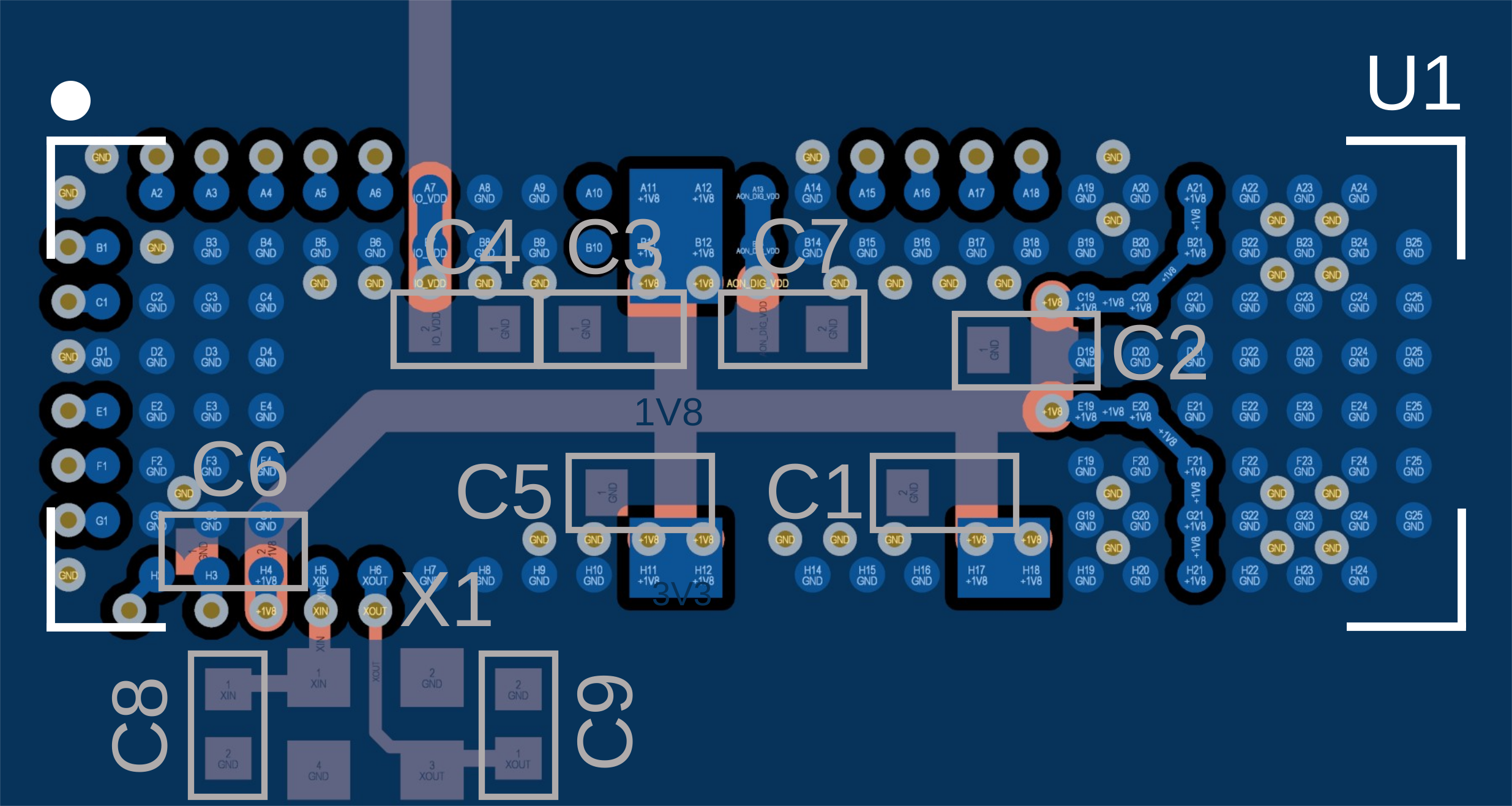
_images/A212_pcb_back_side_components.svg — Figure 4 Example PCB layout with decoupling and crystal placed on sensor back side.#

Ground plane size#

As the ground plane size is increased, the directivity increases because of the larger reflector size. However, the directivity does not increase monotonically with ground plane size due to constructive and destructive interference. For PCBs smaller than 20×15 mm, the H -plane side lobe level increases, which should be considered in applications where this is important.

Radome and mechanical design#

A radome is the product housing or plastic cover in front of the radar that protects it from mechanical impact and weather, see Figure 5. When designed correctly, the radome is effectively transparent to the radar signal and thus not impacting the radiated performance.

Transmission and reflection#

When an electromagnetic (EM) wave hits the interface between two dielectrics, such as plastic and air, reflection and refraction occur at the boundary. Inside the dielectric, the propagation speed and wavelength change depending on the material’s permittivity. If the wavelength in free space is \(\lambda_{0}\), 5 mm at 60 GHz, the wavelength inside the material is \(\lambda=\frac{\lambda_{0}}{\sqrt{\varepsilon_r}}\), where \(\varepsilon_r\) is the relative dielectric constant of the material.

In the case of linearly polarized propagation at normal incidence, the Fresnel equations relate the ratio between the incident and transmitted fields:

(1)#\[r=\frac{Z_{2} - Z_{1}}{Z_{2} + Z_{1}}, \quad t=\frac{2Z_{2}}{Z_{2}+Z_{1}},\]

where \(Z_{1}\) and \(Z_{2}\) are the corresponding wave impedances. The transmission and reflection factors are also related by \(t = 1 + r\). In most cases, we have non-magnetic materials so that \(Z = \sqrt{\frac{\mu_{r}}{\varepsilon_r}} = \frac{1}{\sqrt{\varepsilon_r}}\). An important special case is normal incidence between air and a dielectric. The reflection coefficient then simplifies to

(2)#\[r=\frac{1 - \sqrt{\varepsilon_r}}{1 + \sqrt{\varepsilon_r}}\]

From this expression, we can see that the materials with a higher dielectric constant produce stronger reflections of the incidence signal. Conductors, such as metal, have a very high dielectric constant (\(\varepsilon_r \rightarrow \infty\)) and thus produce a strong reflection. Most polymers have a dielectric constant in the range 2–4, and therefore give a weaker reflection.

Radomes#

Radome thickness#

Let \(d_1\) be the distance to the radome, \(d_2\) the thickness, \(r_1\) and \(r_2\) the reflection coefficients, and \(t_1\) and \(t_2\) the corresponding transmission coefficients according to Figure 5. As an incident wave hits the first interface, a reflection \(r_1\), and a transmission \(t_1\) occur. Note that \(r_1 < 1\), so the reflected wave is out of phase with the incident wave. At the second interface, another reflection \(r_2\) and transmission \(t_2\) take place. With air on both sides of the dielectric, note from Eq. 1 that \(r_1 = -r_2\). The total reflection coefficient \(\Gamma_1\) then becomes [1]:

(3)#\[\Gamma_{1}=\frac{r_{1} \left(1 - e^{-2jkd_{2}}\right)}{1 - r_{1}^{2} e^{-2jkd_{2}}}\]

where \(k = 2\pi/\lambda\) is the wave number in the material. Two notable special cases follow:

For \(d_{2} = m\frac{\lambda}{2}, \; m = 1,2,...\) we have \(e^{-2jk d_{2}}=1\) and \(\Gamma_{1} = 0\).
For \(d_{2} = m\frac{\lambda}{4}, \; m = 1,3,5,...\) we have \(e^{-2jk d_{2}}=-1\) and \(\Gamma_{1} = \frac{2r_{1}}{1+r_{1}^{2}}\).

The optimum radome thickness occurs when the dielectric is perfectly reflectionless, i.e. when the thickness is a multiple of half a wavelength. This can also be understood from the fact that the round trip of the wave inside the radome introduces a 360° phase shift, thereby cancelling the reflected wave \(r_{1}\).

_images/radome_transmission_and_reflection.svg — Figure 5 Transmitted and reflected signals from a half-wavelength radome. Secondary reflections have been omitted for simplicity.#

As an example, if the material is polycarbonate with relative permittivity \(\varepsilon_r=2.75\), the optimal radome thickness becomes:

(4)#\[d_{2}=m\frac{\lambda}{2} = m\frac{\lambda_{0}}{2\sqrt{\varepsilon_r}} = m\frac{5}{2\sqrt{2.75}} \approx m \times 1.51 \:\mathrm{mm}, m = 1,2,...\]

If the dielectric thickness is an odd multiple of \(\frac{\lambda}{4}\), maximum reflection occurs. The relative dielectric constant of some more materials can be found in Table 3.

Dielectric constant of common materials#

The dielectric constant of some common polymers at 60 GHz is presented in Table 3.

Table 3 Relative permittivity of common materials [2]#
Material	Re(\(\varepsilon\)) at 60 GHz
Acrylic glass	2.5
Alumina	9.3
Fused Quartz	3.8
MACOR	5.5
PEEK	3.12 [3]
PMMA	2.6 [4]
Polycarbonate (PC)	2.75 [4] [5]
Polyethylene (PE)	2.3 [5] [6] [7] [8]
Polypropylene (PP)	2.2 [5] [8]
Polystyrene (Rexolite)	2.5
PTFE (Teflon)	2.05 [5]

Footnotes

Disclaimer#

The information herein is believed to be correct as of the date issued. Acconeer AB (“Acconeer”) will not be responsible for damages of any nature resulting from the use or reliance upon the information contained herein. Acconeer makes no warranties, expressed or implied, of merchantability or fitness for a particular purpose or course of performance or usage of trade. Therefore, it is the user’s responsibility to thoroughly test the product in their particular application to determine its performance, efficacy and safety. Users should obtain the latest relevant information before placing orders.

Unless Acconeer has explicitly designated an individual Acconeer product as meeting the requirement of a particular industry standard, Acconeer is not responsible for any failure to meet such industry standard requirements. Unless explicitly stated herein this document Acconeer has not performed any regulatory conformity test. It is the user’s responsibility to assure that necessary regulatory conditions are met and approvals have been obtained when using the product. Regardless of whether the product has passed any conformity test, this document does not constitute any regulatory approval of the user’s product or application using Acconeer’s product. Nothing contained herein is to be considered as permission or a recommendation to infringe any patent or any other intellectual property right. No license, express or implied, to any intellectual property right is granted by Acconeer herein.

Acconeer reserves the right to at any time correct, change, amend, enhance, modify, and improve this document and/or Acconeer products without notice. This document supersedes and replaces all information supplied prior to the publication hereof.

In our code you might encounter features tagged “experimental”. This means that the feature in question is an early version that has a limited test scope, and the API and/or functionality might change in upcoming releases. The intention is to let users try these features out and we appreciate feedback.