Obstacle detection

Obstacle detection#

The Obstacle Detector is an example of a simple obstacle detection algorithm based on the synthetic aperture radar (SAR) principle. The main goal of the obstacle detector is to find obstacles in front of the sensor and estimate their distance and angle. In an application where the sensor is installed on a robot (such as vacuum cleaners or lawn mowers), the object data can be used to issue movement commands to the robot to avoid and circumnavigate the found obstacles. Note that the half power beam width (HPBW) along the H- and E-plane of the sensor is 60 and 40 degrees, respectively.

At the core of the detection algorithm is a fast Fourier transform (FFT), which is used to improve the signal-to-noise ratio (SNR) of obstacles in the vicinity of the radar sensor for extraction of angle \({\alpha}\) and distance \(d\).

Four basic steps are repeated in this algorithm:

Collecting radar sweeps \(s_n\) at a sweep frequency \(f_s\)
Perform FFT of \(N_s\) consecutive sweeps and estimate the power spectral density (PSD)
Perform peak detection on the PSD
Report distance \(d\) and estimate of angle \(\alpha\) for found peak (obstacle)

Sweep collection#

Each radar sweep \(s_n\) consists of \(N_D\) complex delay points, where each delay point represents a specific distance. For moving obstacles, the phase \(\phi\) of its corresponding complex delay point will change based on the sensor-to-object distance change between consecutive sweeps, while the amplitude \(A\) will be unchanged

(20)#\[s_n\left[d_{object}\right] = A e^{i\phi}\]

(21)#\[s_{n+1}\left[d_{object}\right] = A e^{i(\phi+\Delta\phi)}\]

With a sweep frequency \(f_s\) and object velocity \(v_o\), the phase change \(\Delta\phi\) is given by:

(22)#\[\Delta\phi = \frac{4v_o\pi}{f_s\lambda}\]

Note that for Acconeer’s radar module

(23)#\[\lambda = \frac{c}{f_c} = 4.9\,\text{mm}\]

where \(c\) is the speed of light in vacuum and \(f_c\) the radar frequency (\(\sim60\,\text{GHz}\)). During the time the obstacle velocity and angle towards the radar are not changing significantly, the phase change is directly proportional to the number of sweeps \(k\)

(24)#\[s_{n+k}\left[d_{object}\right] = A e^{i(\phi+k\Delta\phi)}\]

On the other hand, for static background amplitude and phase are constant. Static background usually originates from reflections of enclosure or other parts attached close to or in front of the sensor.

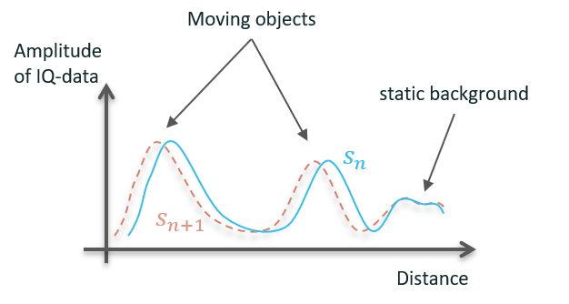
Next, we create a sweep matrix of \(N_s\) consecutive sweeps (17 in our example) as shown in below figure. Time progresses along the x-Axis, distance along the y-Axis. Increasing \(N_s\) will improve angular resolution, but only as long as the obstacle velocity and angle towards the sensor are constant. Reducing \(N_s\) will decrease angular resolution, but also reduce influence of velocity and angle change.

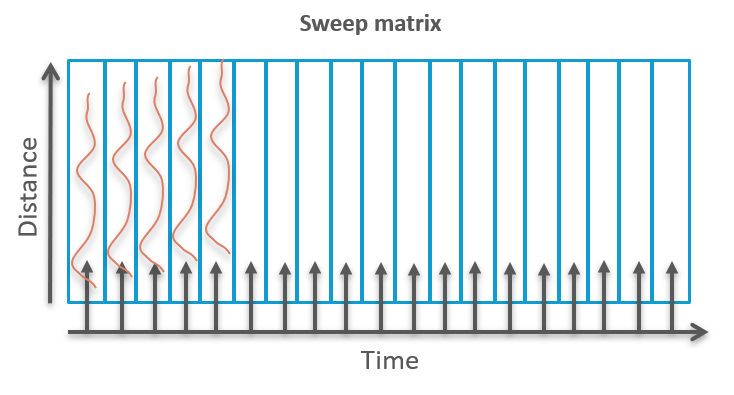
Once the sweep matrix is filled, it will be further processed with each following sweep to extract angle and distance from potential obstacles.

FFT and PSD#

The FFT is performed along the x-Axis of the 2 dimensional sweep matrix, i.e. along the time axis. Thus, each bin \(b\) of the \(N_s\) bins along the x-Axis represents a frequency related to a specific phase change \(\Delta\phi\)

(25)#\[\Delta\phi = b \frac{2\pi}{N_s}\]

Note that \(b\) starts at \(0\) and stops at \(N_s - 1\), thus, phase changes of \(0\) and \(2\pi\) will both appear in bin \(b = 0\). Knowing the relation between bins along the x-Axis of the FFT matrix and the phase change \(\Delta\phi\), we can interpret each bin as velocity according to Eq. 22

(26)#\[v_o = \frac{\Delta\phi f_s\lambda}{4\pi} = \frac{bf_s\lambda}{2N_b}\]

When computing the FFT, delay points of a moving object will coherently add for the bin with the matching phase shift, resulting in an increased amplitude. For all other delay points and other bins, the complex addition of random phase will result in significantly reduced amplitudes compared to the amplitude in the original sweeps. To visualize this concept, the python example calculates the power spectral density (PSD), i.e. the amplitude squared of the complex-valued FFT matrix.

Note that generally obstacles can move towards or away from the radar sensor (or the sensor towards or away from objects). Hence, a phase shift from \(0\) to \(\pi\) is here considered as a “positive” velocity and a phase shift from \(\pi\) to \(2\pi\) as a “negative” velocity (the sign is arbitrarily chosen). Consequently, only phase shifts of up to \(\pi\) can un-ambiguously be attributed to a velocity and the maximum resolvable velocity \(v_{max}\) is given for \(\Delta\phi = \pi\) with Eq. 26 by

(27)#\[v_{max} = \frac{f_s\lambda}{4}\]

For special cases, where only one direction of motion occurs, this can be extended to \(2\pi\). Thus, an FFT shift is performed to “sort” the bins in a way that \(0\) phase shift and velocity is centered and negative and positive velocities extend to the left and right, respectively.

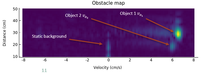
In the python example, the x-Axis of the FFT matrix already shows velocity, ranging from \(-v_{max}\) to \(+v_{max}\). It uses by default a sweep frequency \(f_s=66\,\text{Hz}\) resulting in a maximum resolvable velocity \(v_{max}=\pm8\frac{\text{cm}}{\text{s}}\). Around \(0\frac{\text{cm}}{\text{s}}\) velocity, some signal is visible originating from enclosure of the sensor. This static signal is fixed in amplitude and position. To the right, at a velocity of \(6\) to \(7\frac{\text{cm}}{\text{s}}\) we see 2 distinct peaks coming from 2 different objects at around \(20\) and \(30\,\text{cm}\).

To visualize the coherent addition of sweeps at the matching bin, the example also shows the envelope of the current complex sweep (blue solid line) and the envelope along the bin of the global maximum in the FFT matrix (dashed orange line).

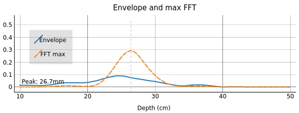
The bin with the global peak is here around \(7\frac{\text{cm}}{\text{s}}\). As can be seen, the signal-to-noise ratio (SNR) of the peak to the rest of the sweep has increased significantly. While we use the FFT information mainly for extracting an angle (see step 4), a major advantage of this method is the improved signal (SNR) and thus significantly lowered detection threshold.

Peak detection#

The example uses the most basic peak detection, which only identifies the global maximum. With a more advanced implementation, local maxima could also be identified so that multiple obstacles may be reported simultaneously. Each found peak is interpreted as an obstacle at a certain distance (y-Axis) with a certain velocity (x-Axis). It should be noted that it might be necessary to employ background subtraction or restricting peak-finding to bins corresponding to non-zero velocity in order to exclude peaks from static objects or general noise in the FFT.

Distance and angle#

In the final step, the example calculates the angle \(\alpha\) the obstacle has with respect to the sensor. In order to do so, we need to assume that either the sensor is moving and all found obstacles are motionless or vice versa. In general, when the sensor and the obstacles are moving at the same time, the measured phase shift cannot be related un-ambiguously to a velocity according to Eq. 22 and hence no statement about the obstacle’s angle can be made.

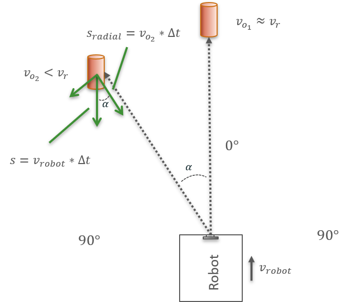
We assume that the radar sensor is moving at a constant velocity \(v_{robot}\) (being attached to a robot) and all obstacles are motionless. Thus, in the reference frame of the sensor, all obstacles are moving with \(v_{robot}\) towards the robot parallel to the normal of the robot front. In this example we set the robot velocity to

(28)#\[v_{robot} = v_{max} = \frac{f_s\lambda}{4}\]

Note that between consecutive sweeps

(29)#\[\Delta t = \frac{1}{f_s}\]

the robot travels a fixed distance \(\Delta s\) of

(30)#\[\Delta s = v_{robot}\Delta t = \frac{\lambda}{4}\]

In order to calculate the angle \(\alpha\) of the obstacle with respect to the sensor, we need to resolve the obstacle’s velocity vector into its radial and tangential component (as shown in above figure) such that

(31)#\[\vec{v}_{obstacle} = \vec{v}_{robot} + \vec{v}_{o_i}\]

The velocity \(v_{0_i}\) of obstacle \(i\), measured with the FFT matrix, is the radial component of \(v_{robot}\) with respect to the object. From this we can calculate \(\alpha\) using

(32)#\[\alpha = \cos^{-1}\left(\frac{v_{o_i}}{v_{robot}}\right)\]

For calculation of the actual value of \(\alpha\), we need to substitute the velocities with bins (along the x-Axis of the FFT matrix) and consider that half the bins are for positive and the other half for negative velocities. We thus get for the obstacle bin \(b_{o_i}\)

(33)#\[v_{o_i} = \frac{b_{o_i}}{N_s/2}\frac{\lambda f_s}{4}\]

and for the robot bin \(b_{robot}\)

(34)#\[v_{robot} = \frac{b_{robot}}{N_s/2}\frac{\lambda f_s}{4}\]

which results in

(35)#\[\alpha = \cos^{-1}\left(\frac{b_{o_i}}{b_{robot}}\right)\]

Note that in this example, since we set \(v_{robot}\) to be \(v_{max}\), the bin matching the robot velocity is

(36)#\[b_{robot} = \frac{N_s}{2}\]

Finally, if the example finds an obstacle in the FFT matrix, it prints the obstacle distance, velocity and angle at the lower left side of the FFT matrix, taking above assumptions into account.

Configuration parameters#

class acconeer.exptool.a111.algo.obstacle_detection._processor.ProcessingConfiguration#

fft_length#: Type: int

Default value: 16

threshold#: Type: float

Default value: 0.05

downsampling#: Type: int

Default value: 1

calib#: Type: int

Default value: 10

bg_offset#: Type: float

Default value: 1.6

static_threshold#: Type: float

Default value: 0.1

close_threshold_addition#: Type: float

Default value: 0.1

static_distance#: Type: float

Default value: 45

static_grad#: Type: float

Default value: 6

close_dist#: Type: float

Default value: 16

static_freq#: Type: float

Default value: 2

nr_peaks#: Type: int

Default value: 1

edge_to_peak#: Type: float

Default value: 1

peak_hist#: Type: int

Default value: 500

robot_velocity#: Type: float

Unit: cm/s

Default value: 6

use_parameterization#: Type: bool

Default value: False

background_map#: Type: bool

Default value: True

threshold_map#: Type: bool

Default value: False

show_line_outs#: Type: bool

Default value: False

velocity_history#: Type: bool

Default value: True

angle_history#: Type: bool

Default value: True

distance_history#: Type: bool

Default value: True

amplitude_history#: Type: bool

Default value: True

sensor_separation#: Type: float

Unit: cm

Default value: 15