Tank level short (envelope)

The intention with this processor is to solve the problem of detecting a fluid level in a small tank. It does so by estimating the distance from the radar to the closest reflecting surface.

Depending on the tank geometry and/or the configured detection distance, a calibration might be required for relevant results. At distances closer than 5 cm, the measured value might not be accurate. However, an internal ranking of distances should still work at close ranges (i.e. an object at a distance of 2 cm is reported as closer than an object at a distance of 3 cm, which is reported as closer than an object at 4 cm).

Calibration

It is strongly recommended to use a calibration, if this step is ignored, the output will be poorly scaled, although there is nothing in the code that prevents usage or warns if the calibration step is skipped. It will only be reflected by poor results. The calibration is normally done “open-air”, which means that the sensor should not be pointed at anything when calibrating. However, erroneous distance reports can be observed if the geometry of the intended target is prohibitive. So it is always a good idea to evaluate calibration with the sensor in it’s intended position (i.e. in the tank) as well.

To calibrate the sensor using exploration tool, start measurement and wait 50 frames. After that, press the “Apply Calibration” button in the calibration section.

Data processing

Data is processed by first applying a calibration, which subtracts the background noise and any static reflections if the calibration was done “in tank”. The calibrated data is scaled by the normalized distance to the sensor and then normalized over the frame. The normalized value is filtered by an exponential filter with an adjustable time constant (called smoothing time const).

\[scaled\_data = calibrated\_data * scale\_array\]

\[norm\_data = scaled\_data / max(scaled\_data)\]

\[smooth\_val = smooth\_val * smooth\_const + (1.0 - smooth\_const) * norm\_data\]

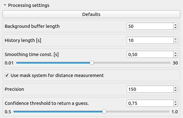
There are then two processing options: “Basic” and “Masks”. The different options can be toggled with the “Use mask system for distance measurement” check box found in the exploration tool interface.

Figure 55 Check box to toggle distance calculation type.

The “Basic” system just finds the maximal amplitude in the smoothed normalized value and returns the index of the max value. The mask matching is more sophisticated and resource intensive. It is recommended to start evaluate the performance of the “Basic” system before using the mask system.

Mask Matching

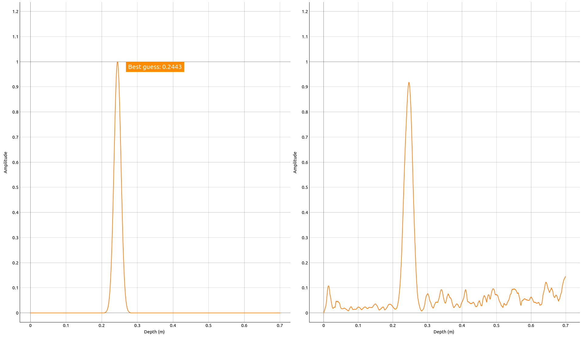
Depending on the desired precision, a number of “masks” are generated at startup. A mask is an array of the same dimensions as the input data, representing an idealized profile of an object at a given distance. All masks are generated at startup, for full details, it is recommended to investigate the source code. The function responsible for generating the masks is called “calculate_mask”. The filtered data is matched against all masks and given a score. The corresponding distance for the mask with the best matching score is returned if the matching score is above a threshold.

Figure 56 Example of a mask (left) with a high matching score and the processed sensor data (right).

Low threshold will yield reported distances even when there is nothing in front of the sensor. A high threshold could cause nothing to be reported, it is recommended to evaluate by adjusting the threshold to the lowest setting. If a return value always is expected (i.e. there is always something in front of the sensor) then it is recommended to use the lowest threshold setting.

Mask score

To obtain the score, we first estimate the missed amplitude over all depths. The missed amplitude is calculated by:

\[miss = max(mask, data) - min(mask, data)\]

For each mask, the sum is then divided by the total number of depths (i.e. assuming an amplitude of 1.0 for all depths). The final score is obtained by:

\[score = 1.0 - sum(miss)/len(data)\]

A mask of 1.0 everywhere and an empty data array would thus get a score of 0.0 and a perfect match would get a score of 1.0

Score Threshold

The best scoring mask has the score compared against a threshold, if the check fails, nothing is returned. This is to avoid returning varying guesses for an empty channel. However, the best masks for detection close to the sensor might have a lower score than a mask matching against an empty channel. So beware and try to evaluate cases on lower thresholds.

Precision

This variable decides how many masks the algorithm should check against. This directly decides how many possible values the output can have. For example, a precision of 2 would only yield two masks (at the start and end of your range), so the output can only have one of these two values. Higher value yields more possibilities within the range but slower performance (since we need to calculate a score for each of these possibilities for each data frame).