Speed (sparse)#
This is a speed measuring algorithm built on top of the Sparse service – based on measuring changes in the radar response over time. The algorithm calculates a speed estimate of a target’s radial speed from or towards the sensor.
Plots#

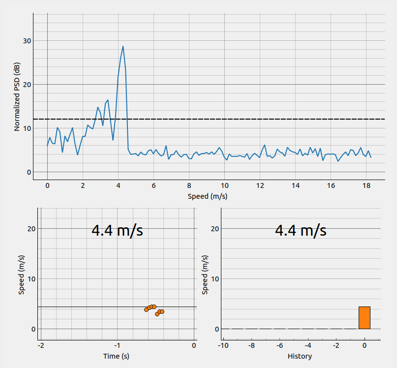
Figure 80 A screenshot of the plots. A target detected with the speed 4.4 m/s can be seen.#
Top plot: The plot shows the normalized power spectral density (PSD) for a frame in dB on the y-axis and speed in m/s on the x-axis. The dotted black line marks the threshold level set in Processing settings.
Lower left plot: The scatter plot shows all points which surpass the threshold in the top plot. The black line marks the point with the greatest speed.
Lower right plot: The plot illustrates the the latest top speeds in a bar graph. There must be approximately 0.5s between two point clusters to make the graph register a new top speed.
Detailed description#
The Sparse service returns data frames in the form of \(N_s\) sweeps, each consisting of \(N_d\) range depth points, normally spaced roughly 6 cm apart. We denote frames captured using the sparse service as \(x(f,s,d)\), where \(f\) denotes the frame index, \(s\) the sweep index and \(d\) the range depth index. As described in the documentation of the Sparse service, small movements within the field of view of the radar appear as sinusoidal movements of the sampling points over time. Thus, for each range depth point, we wish to detect changes between individual point samples occurring in the \(f\) and \(s\) dimensions.
Speed estimation#
The speed estimation algorithm is based on the power spectral density of the radar signal. Welch’s or Bartlett’s method is used to estimate this PSD.
The estimation is carried out by dividing the sweeps for each distance into segments, then forming a windowed periodogram of each segment and averaging all segments together.
The m:th windowed and zero-padded segment from the signal x can be denoted by
where R is defined as the segment size, \(w(n)\) is defined as the window function and K is defined as the number of segments. The periodogram of the m:th segment is given by
The power spectral density estimation is then given by
which calculates the average of the periodograms.
In Processing settings the estimation method can be chosen as either Welch’s or Bartlett’s method. In Welch’s method the overlap of the segments are 50% and the used window, \(w(n)\), is a Hann window. In Bartlett’s method the segments does not overlap and \(w(n)\) is a rectangular window, which results in a non-modified periodogram. Welch’s method will result in lower variance, less leakage but decreased resolution compared to Bartlett’s method.
When the estimated PSD is attained by the methods above, the speed can easily be derived from its frequency contents. A period of a sinusoid in the data corresponds to an object having moved a perceived wavelength of the radar, i.e., ~2.5mm. So, for example, if we see a sinusoid with a frequency of 1kHz, we can calculate that this corresponds to a speed of 1000 Hz * 0.0025m = 2.5m/s.
Graphical overview#
Configuration parameters#
- class acconeer.exptool.a111.algo.speed_sparse._processor.ProcessingConfiguration#
- class ProcessingMethod(*values)#
- threshold#
The threshold parameter determines how great PSD a point needs to have to be included in the speed estimation. The threshold value is converted to dB when displayed in the Normalized PSD-graph
Type: floatDefault value: 4.0
- min_speed#
The minimum speed to be displayed.
Type: floatUnit: m/sDefault value: 0.5
- fft_oversampling_factor#
- Type: intDefault value: 1
- processing_method#
In Welch’s method the segments overlap 50% and the periodograms are windowed using a Hann window. In Bartlett’s method there is no overlap between segments and the periodograms are not modified. Welch’s method will result in lower variance and added complexity compared to Bartlett’s method.
Default value: ProcessingMethod.WELCH
- num_segments#
Number of segments used in Welch’s/Bartlett’s method.
Type: intDefault value: 3
- shown_speed_unit#
- Default value: SpeedUnit.METER_PER_SECOND
- show_data_plot#
- Type: boolDefault value: False
- show_sd_plot#
- Type: boolDefault value: True
- show_vel_history_plot#
- Type: boolDefault value: True
- num_shown_sequences#
Number of bars to be displayed in the bar graph
Type: intDefault value: 10